What Is a WAV File
WAV is an audio file format, or more specifically, a container format to store multimedia files. It is formerly known as WAVE (Waveform Audio File Format), and referred to as WAV because of its extension (.wav or sometimes .wave). The initial release of WAVE was in August 1991, and the latest update is in March 2007.
WAV and WAVE are used interchangeably to refer to the same thing. It was developed jointly by Microsoft and IBM. In fact, it is a subset of Microsoft's RIFF (Resource Interchange File Format) standard, which stores data in chunks.
What Is RIFF that WAV Based on
RIFF (Resource Interchange File Format) is a container format to store data and is widely used for many kinds of multimedia files on Windows. The file format is signified by its extension. For instance, Audio-Video Interleaved (.AVI), MIDI files (.RMI), color palette files (.PAL), animated mouse cursors file format (.ANI), and Waveform audio file format (.WAV) are all based on RIFF.
RIFF stores data in chunks and the chunks are tagged to be identifiable. Since WAV is also based on RIFF, it shares the way the chunks are tagged. You will learn more of its structure later in this post.
How to Open WAV files
Since WAV is an audio file, media players that support WAV format will be able to open and playback WAV files, including the default Windows Media Player, and iTunes, and QuickTime Player on Mac. Open-source media players such as VLC also support the format.
If you want to analyze the files structure of WAV files, you can use code editors to open the file.
WAVE Specifications: What Is the File Structure of WAV
To understand how is WAV encoded and stored, we can look at its file structure. Since the WAVE file is a substance or a subset of the RIFF file, it inherits the file structure of RIFF.
Just as the RIFF file that consists of the file header at the start, and followed by several data chunks, WAVE starts out with a file header, which requires two subchunks "fmt " and "data" (note there is a space after fmt), and the data chunk, which includes the ID and size of the data, and the actual raw data of the audio.
Canonical WAV File Structure
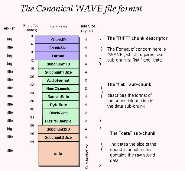
Below is an illustration of the file structure of the canonical WAV file format that stores PCM data.
Note:
- Offset: indicates where that field should start. For instance, information of ChunkSize is stored in 04 05 06 07; and information of Subchunk1ID is stored in 12, 13, 14, 15.
- Endianness: the order of the bytes stored in memory, when that value takes up multiple bytes. Big endian puts the largest byte first, and little endian does the opposite.
- The file header is 44 bytes.
Non-PCM WAV File Structure
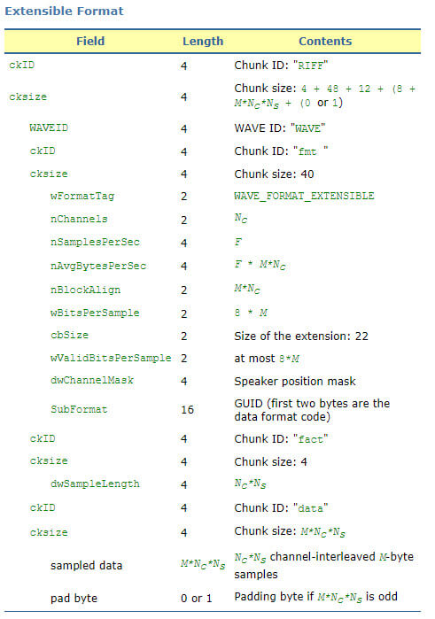
Below is the file structure of WAV file storing non-PCM data. As you can see, an extended format chunk is used in the structure.
Note:
- For non-PCM data, the size field must be included in the structure, even if the extension is zero length.
- A fact chunk must be present for non-PCM data.
- For a more detailed explanation, please refer to Audio File Format Specifications.
Understanding the WAV File Structure: Analysis of a WAV Sample
To better understand the structure, let's analyze a sample WAV file.

00-03: Hexadecimal representation of the ASCII form of the letters "RIFF". Therefore, it is always the same for all WAV files: 52 49 46 46.
04-07: Size in bytes from 08 to the rest of the file. The value of it plus 8 bytes (the size of 01 to 07) is the file size of the WAV file.
Let's do simple math:
- Already known sample file size: 2,646,044 bytes.
- 04-07 value: 14 60 28 00; Little endian: 00 28 60 14; headecimal to decimal: 2,646,036.
- As you can see, adding 8 bytes to 2,646,036 equals the file size of the sample WAV file.
08-11: Hexadecimal representation of the ASCII form of the letters "WAVE". Therefore, it is 57 41 56 45 for every WAV file.
12-15: Indicates the letter "fmt " (note the blank space here), which is always 0 x 66 6d 74 20, and 0x20 corresponds to the blank space.
16-19: subchunk size 16, that is the sum of the rest subchunk size from audio format to BitsPerSample (2+2+4+4+2+2=16).
20-21: Audio format, 1 for PCM, other values represent other forms of compression. Litter endian, so the hexadecimal 0001 is 1 in decimal.
22-23: Number of channels. 1 for mono, 2 for stereo.
24-27: Sample Rate (Sample per second). 00005622, 22050Hz. FYI, 80 BB 00 00 stands for 48000 Hz (little endian 0000BB80);
28-31: Average Bytes Per second (ByteRate). ByteRates=(Sample Rate x Bits Per Sample x Channel Numbers)/8
32-33: Block Align: Data block size.
34-35: Bits per sample: 16bits=1000 (little endian 0010); 32bits=2000 (little endian 0020); etc.
36-39: Hexadecimal representation of the ASCII form of the letters "DATA".
40-43: Number of bytes in the data, which equals: (Sample numbers x Channel numbers x Bits per sample)/8
PCM and WAVE
PCM, short for Pulse Code Modulation, is a method to capture waveforms and store the audio waveforms digitally. It is the base for all audio formats, and when it stores raw, such as using the WAV container, it is known as lossless audio.
We know that the sound in the physical world is a form of wave, or more specifically, the sine wave. It is a continuous function, meaning there are no breaks even within the tiniest time intervals. To sample it, you cannot capture every point since there are infinite numbers of points that form the waveform.

So, instead of capturing the infinite numbers of points digitally to represent the wave, the concept is to sample points at regular time intervals, then go through some mathematical process to reproduce a waveform that is identical to the real world one, based on those samples.

The aim here is to save only enough points to closely resemble the real world wave function. To better understand the idea, let's go through the process from sampling, quantization, to encoding, with terms such as sample rate, bit depth, and bitrate explained.
How to Digitally Measure the Wave Over Time: Sample Rate
Hertz is the frequency that tells you how many circles (or periods of the sine form) are there in one second. On the left picture, there is only one circle in 1 second, so it is 1 Hz; On the right, it is 5 Hz.
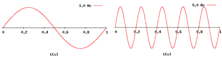
As explained above, the digital method is to save enough points to resemble the physical world waveform. The practice of taking regular measurements (the points) throughout a cycle is called sampling Rate. For instance, 44.1kHz (44100 Hz), commonly seen in audio projects, is a sampling rate that captures 44100 points in a second from the wave.
How to Ensure There Are Enough Samples
The question can also be asked this way, why do we use 44.1kHz as the main consumer standard? It has to do with the Nyquist-Shannon theorem, which states that the sampling rate must be at least double the rate of the highest frequency (fs.max>=2Fmax).
Human ear can detect sounds in a frequency range from about 20Hz to 20kHz. So in a 44.1kHz sampling rate project, there are 20 circles in one second for the lowest pitch 20Hz, measured by 44100 points; and 20,000 circles in one second for the highest pitch 20kHz, sampled by 44100 points, meaning there are more than 2 points in one circle. Therefore, 44.1kHz is more than doubling the rate of the highest frequency (20kHz) perceivable by human ear.
As we already know, the theorem is a non-self-evident proposition that is proved to be true by other accepted statements or a chain of reasoning. You can watch the Sampling Theorem (5:35) from Digital Audio Fundamentals Series, where Akash Murthy experiments sampling less than double of the highest frequency and many other situations.
There are other sampling rates such as 48kHz, 88.2kHz, 96kHz, 192kHz depending on the project you are working on, and the hardware setup.
How to Digitally Represent the Amplitude of the Analog Audio: Bit Depth
Now we know that the horizontal axis has to do with the sampling rate. How about the vertical axis?
Let's consider the situation of using four levels (2bit) to quantify the audio amplitude versus using 16 bit.

Since the computer knows only 1s and 0s:
- 1 bit is either 0 or 1;
- 2 bit: 00, 01, 10, 11;
- 3 bit: 000, 001, 010, 011, 100, 101, 110, 111;
- 16 bit: there are 65536 possible vertical axis values (2^16=65536).
- 24 bit has over 16 million values (2^24=16777216).
As you can see, higher bit depth, together with a higher sample rate measured over time, result in a more precise model.
Audio Quantization
Since the modeling is a discrete function, as opposed to the continuous wave happening in the real world, we can see that some points on the wave don't fall on the grit provided by bit depth. The mathematical solution is to move that point to its nearest point inside the grit. The process is known as quantization.
It is obvious that higher bit depth and sample rate make the quantization produce results closer to the real situation.
Then all these levels/grits are encoded into 0s and 1s for the computer to read.
In Audio engineering, commonly seen bit depths are 16 bit, 24 bit, 32 bit and 32 bit float.
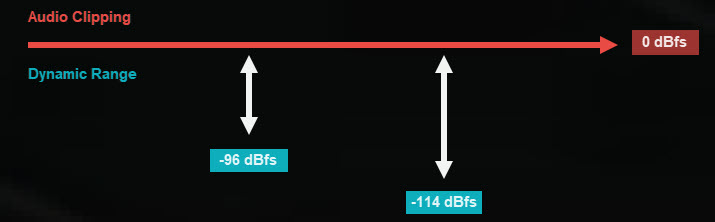
When measured in decibels:
- The dynamic range of 16 bit is 20xlog (2^16)≈96, ranging from -96 dBfs to 0 dBfs
- The dynamic range of 20 bit is 20xlog (2^24)≈144, ranging from -144 dBfs to 0 dBfs
Audio above 0 dBfs will be clipped, you can learn more about this in audio normalizing.
Note:
The quantization process also takes place when converting between bits. For instance, the 24 bit has more depth than 16 bit, interpolating the waveform is needed and then resampling it using the new bit depth.
For us to hear the audio, for instance, the WAV file, it will be converted back from digital to analog through the DAC (digital to analog converter), which is a chip as part of the audio hardware.
Calculating WAV File Size with Bitrate
From the above examples and illustrations, we already know the concept of bit depth and sampling rate. With the value of these two, bitrate can be derived.
Bitrate = sampling rate (samples per second) x bit depth (bits per sample) x number of channels.
ByteRate = Bitrate/8
Note: If the audio is stereo, you need to multiply the above result with the number of channels of the wav file.
WAV vs MP3
MP3 (MPEG-2 audio layer III) is developed by the Moving Picture Experts Group (MPEG). It is a lossy audio format that is compressed and leaves out some data. It reduces data for a smaller file size at the cost of quality, though the difference won't be that large for the human ear to distinguish. It handles the compressing according to psychoacoustics, that is, how the human ear perceives the sound.
For instance, in the raw recordings, there are certain frequencies that cannot be heard by the human ear. The compression leaves out those redundant frequencies. For quieter sounds covered up by louder sounds, the compression gets rid of the data that represents the quieter sounds.
By exploiting these aspects and taking advantage of our perception as opposed to the reality, MP3 compression manages to reduce file size, while still maintaining acceptable sound quality.
While for WAV, as we already covered in the previous part, is a lossless format encoded with PCM. Since it contains the raw data, WAV generally results in a larger file size comparing to MP3. It is ideal for mastering audio, editing the audio file, and store audio files where quality matters over the file size. However, there may be compatibility issues as compared to MP3. For instance, iPhone and iPad don't support WAV natively.